Water bodies detection

This application takes as input Copernicus Sentinel-2 or USSG Landsat-9 data and detects water bodies by applying the Otsu thresholding technique on the Normalized Difference Water Index (NDWI).

The NDWI is calculated with:

\[ NDWI = { (green - nir) \over (green + nir) } \]

Typically, NDWI values of water bodies are larger than 0.2 and built-up features have positive values between 0 and 0.2.

Vegetation has much smaller NDWI values, which results in distinguishing vegetation from water bodies easier.

The NDWI values correspond to the following ranges:

Range	Description
0,2 - 1	Water surface
0.0 - 0,2	Flooding, humidity
-0,3 - 0.0	Moderate drought, non-aqueous surfaces
-1 - -0.3	Drought, non-aqueous surfaces

To ease the determination of the water surface/non water surface, the Ostu thresholding technique is used.

In the simplest form, the Otsu algorithm returns a single intensity threshold that separate pixels into two classes, foreground and background. This threshold is determined by minimizing intra-class intensity variance, or equivalently, by maximizing inter-class variance:

The application can be used in two modes:

take a list of Sentinel-2 STAC items references, applies the crop over the area of interest for the radiometric bands green and NIR, the normalized difference, the Ostu threshold and finally creates a STAC catalog and items for the generated results.

This scenario is depicted below:

graph TB subgraph Process STAC item A[STAC Item] -- STAC Item URL --> B A[STAC Item] -- STAC Item URL --> C A[STAC Item] -- STAC Item URL --> F subgraph scatter on bands B["crop(green)"]; C["crop(nir)"]; end B["crop(green)"] -- crop_green.tif --> D[Normalized difference]; C["crop(nir)"] -- crop_green.tif --> D[Normalized difference]; D -- norm_diff.tif --> E[Otsu threshold] end E -- otsu.tif --> F[Create STAC Catalog] F -- "catalog.json/item.json/asset otsu.tif" --> G[(storage)]

read staged Landsat-9 data as a STAC Catalog and a STAC item, applies the crop over the area of interest for the radiometric bands green and NIR, the normalized difference, the Ostu threshold and finaly creates a STAC catalog and items for the generated results.

This scenario is depicted below:

graph TB subgraph stage-in A[STAC Item] -- STAC Item URL --> AA[Stage-in] AA[Stage-in] -- catalog.json/item.json/assets blue, red, nir ... --> AB[(storage)] end subgraph Process STAC item AB[(storage)] -- Staged STAC Catalog --> B AB[(storage)] -- Staged STAC Catalog --> C AB[(storage)] -- Staged STAC Catalog --> F subgraph scatter on bands B["crop(green)"]; C["crop(nir)"]; end B["crop(green)"] -- crop_green.tif --> D[Normalized difference]; C["crop(nir)"] -- crop_green.tif --> D[Normalized difference]; D -- norm_diff.tif --> E[Otsu threshold] end E -- otsu.tif --> F[Create STAC Catalog] F -- "catalog.json/item.json/asset otsu.tif" --> G[(storage)]

Alice packages the application as an Application Package to include a macro workflow that reads the list of Sentinel-2 STAC items references or Landsat-9 staged data, launches a sub-workflow to detect the water bodies and creates the STAC catalog:

The sub-workflow applies the crop, Normalized difference, Otsu threshold steps:

The development and test dataset is made of two Sentinel-2 acquisitions:

Acquisitions
Mission	Sentinel-2	Sentinel-2
Date	2022-05-24	2021-07-13
URL	S2B_10TFK_20210713_0_L2A	S2A_10TFK_20220524_0_L2A
Quicklook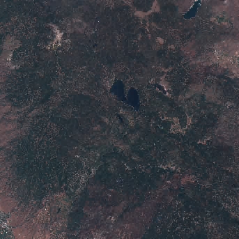

And one Landsat-9 acquisition:

Acquisition
Date	2023-10-15
URL	LC09_L2SP_042033_20231015_02_T1
Quicklook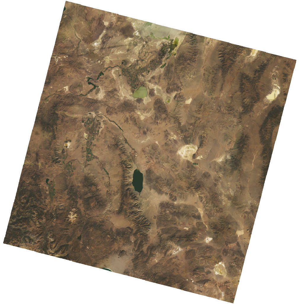

Each Command Line Tool step such as crop, Normalized difference, Otsu threshold and Create STAC runs a simple Python script in a dedicated container.